Annual Daylight Simulation

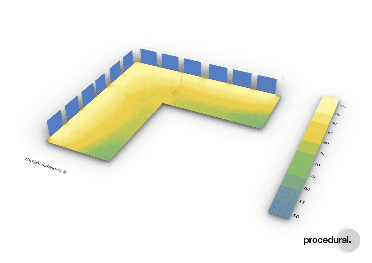
In this tutorial we will go through a step-by-step guide of how to use Compute to run an annual daylight simulation. The end result will be a mesh colored according to the results we get from Daylight Autonomy.

Setup

To follow along or to try it yourself, download our demo file of this tutorial.

Canvas

The Grasshopper canvas looks as the picture below.

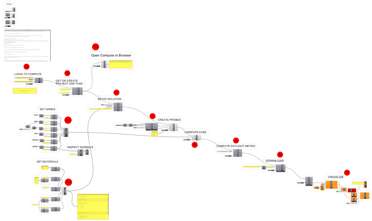
We have 8 steps to go through:

0. Login
1. Project and Task creation
2. Case and Solution Setup
3. Probe Task Creation
4. Simulation Task Creation
5. Daylight Metric Task Creation
6. Download Results
7. Visualize

If you are already familiar with the daylight setup, then we suggest that you skip straight to Assign Materials and Simulation Task Creation

Login

The first thing to do is to log in with your username and password. If you don't have an user for Compute yet, then you need to sign up first. You can go to our registration page to do so.

Project and Task Creation

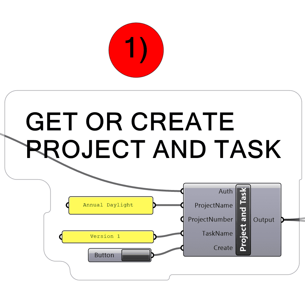
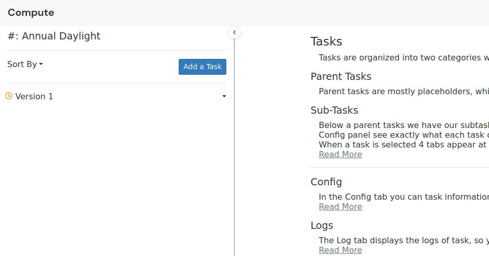
Every task on Compute belongs to a project. Then first thing to do is to create that project. You can do it manually through the web browser or you can do it with the Grasshopper components. Here we are going to stick to the Grasshopper components.

We will call our project Annual Daylight and our TaskName Version 1. The parent task we create together with our project works to group our simulation tasks, so we can easily keep track of design iterations. When we click on the Create button the project and task will be created on Compute.

Case and Solution Setup

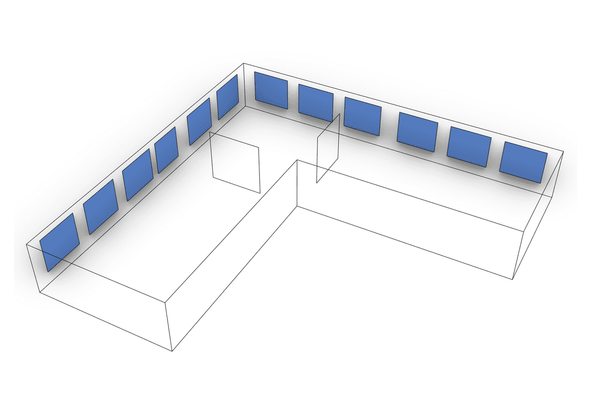
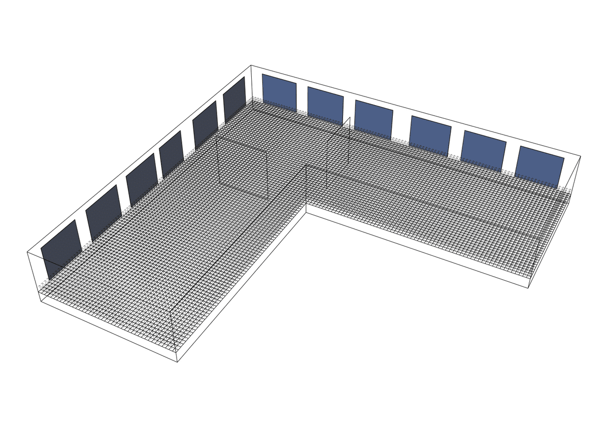
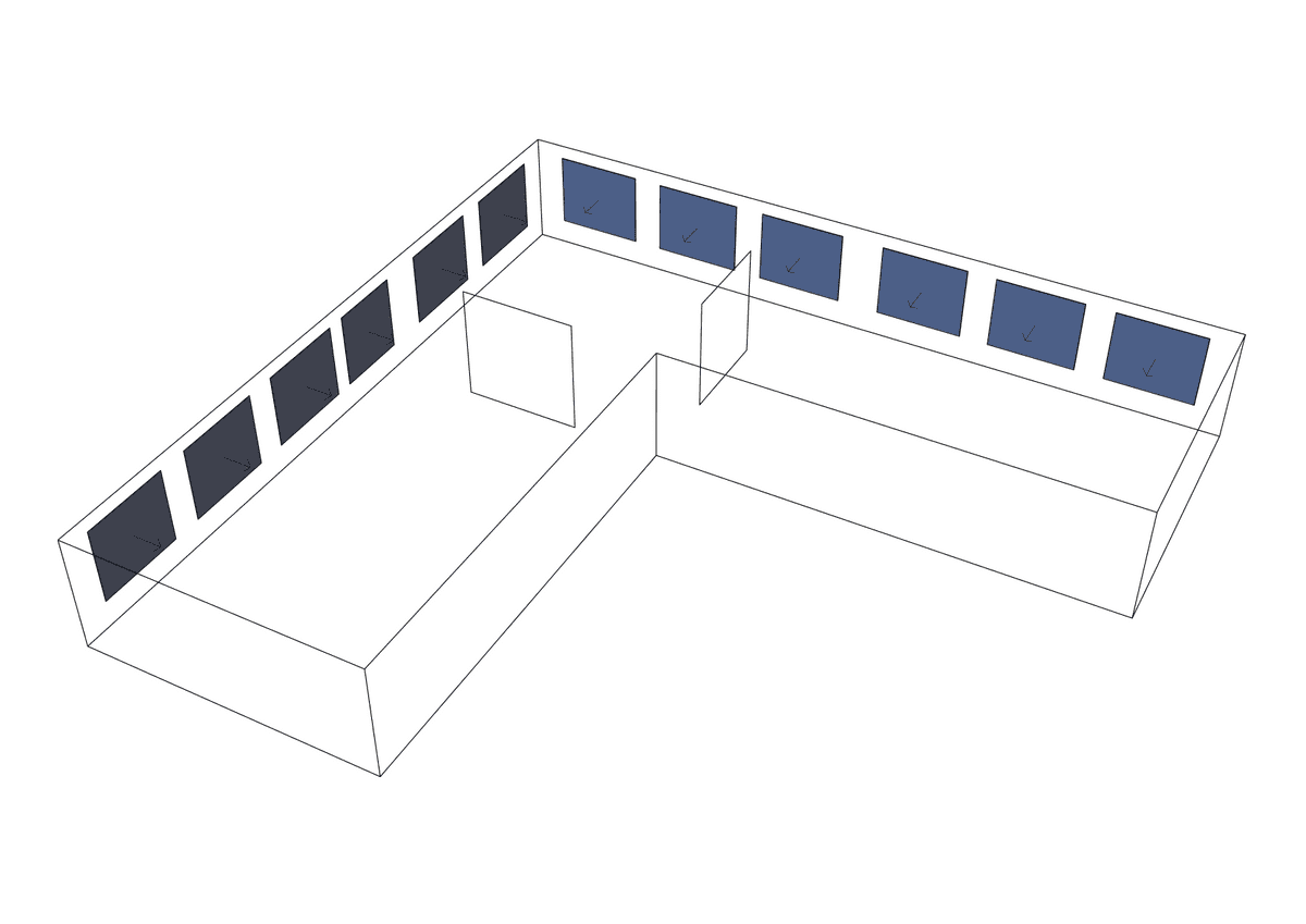
Next thing on the agenda is to set up the case and geometry. In this tutorial we are working with an L-shaped office space that has windows on the north and east facade. We have two interior walls, which splits the office space into three rooms.

Apply Naming

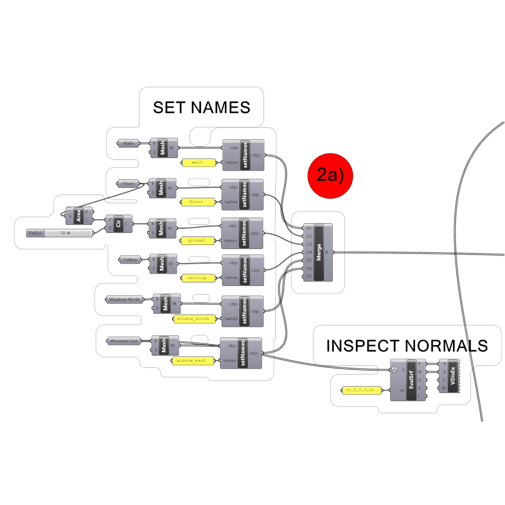
With the Compute Grasshopper plugin we work with the geometry first by naming it. Each surface gets its own name. That way it is possible to assign materials later on. The SetNames components only accepts mesh geometry, that is why we use Grasshopper Mesh Brep component to turn our surfaces into meshes.

We give descriptive names to the surfaces such as wall, floor and window_east. It makes it a lot easier later on figure out what is what.

The SetNames component accepts a list of objs (meshes), but you can choose to only give the names into a single value. That doesn't mean that every surface inputted to objs are i.e. going to be called wall. The component will detect that you gave it a list of meshes, but only a single name and therefore it will suffix the name with a number. So the final outcome looks something like this: wall.__000, wall.__001, wall.__002, wall.__003.

Inspect Geometry

When running Daylight simulations it is important that your geometry is clean and without any gaps, just when doing CFD The simulation engine we use for daylight and radiation is Radiance, which is a validated and widely use simulation engine. Radiance is sensitive to the orientation of surface normals, so you have to make sure that the normal points the way you want, before starting the simulation.

In the demo Grasshopper file, we provide with a simple setup to check the normals of the case geometry. The surface normal should point towards the side you want to ray trace, so in case of the indoor daylight assessment you want the normals to point inward.

Assign Materials

We assign materials to the names of the geometry. On the server the materials and the geometry are matched based on the naming. That is why we need to apply the names to the geometry.

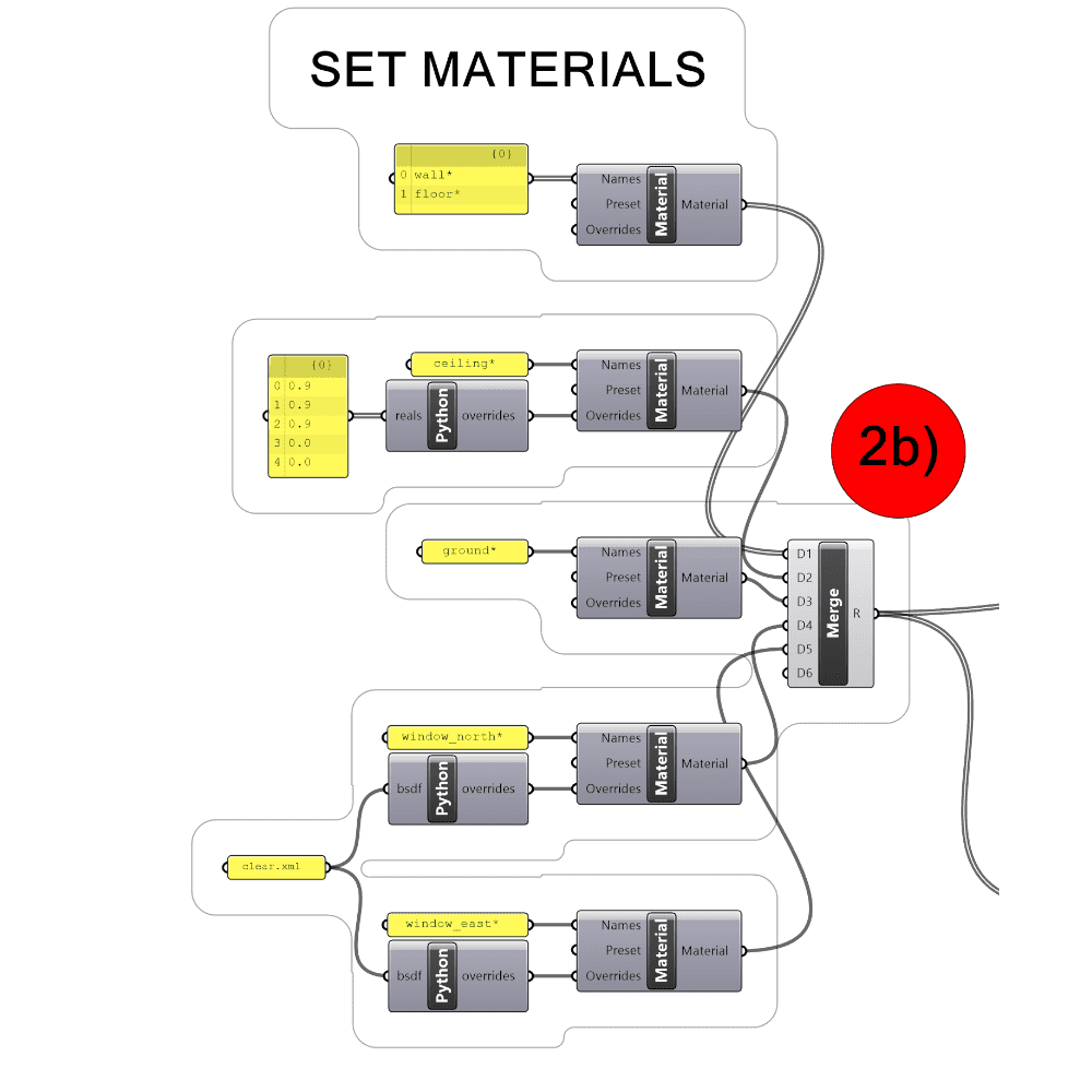
The Material component takes a list of names, a preset and a JSON formatted string with overrides. In the picture below you can see that in the top component we supply the names: wall*, floor*. As you probably noticed, we don't have any geometry named wall* or floor*. The * means that we match everything the starts with wall or floor. We use the * so we don't have to input a list with all the names we assigned earlier. Remember that the SetNames component give the geometry a suffix with a number on. So it could be a quite long list to supply to the Material component. We can avoid all that with the simple * notation.

If you are interested in reading more about the presets and overrides you can choose between, take a look at Radiance Materials

The most important override is the bsdf for the windows. The BSDF file is the Transmission Phase for the 3 Phase Method we use to simulation annual daylight. In the demo we use the clear.xml file, which Compute implements as a demo file. In real, you should create your own BSDF file with the WINDOW software provided by LBNL.

The Python components are a convenient way of turning inputs into JSON formatted text. You can see what is going on inside the component by double-clicking on it.

Setup Solution

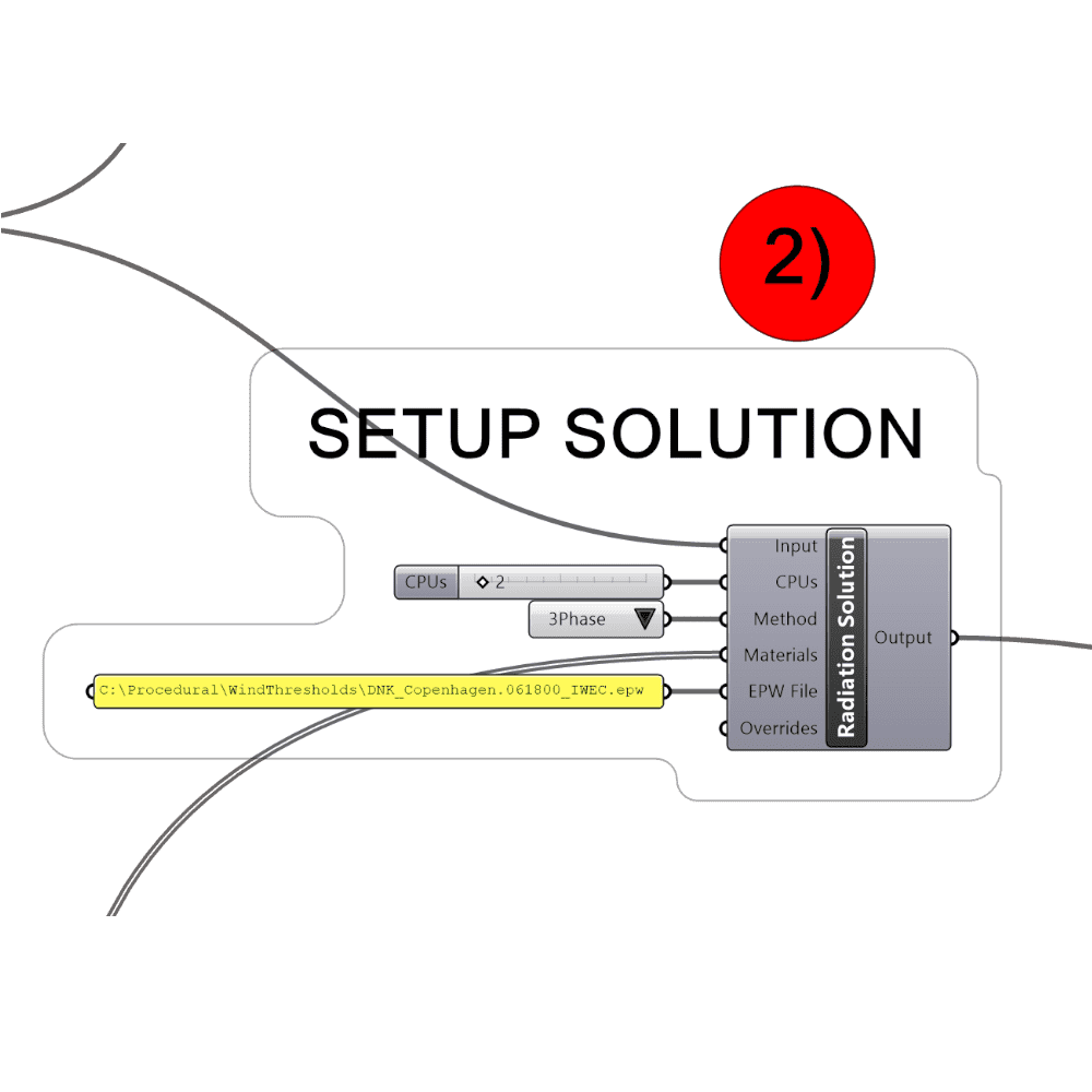
The final part of the case and geometry setup is to configure the Solution component. The solution takes Input from the ProjectAndTask component, that we looked at in the beginning. You further more need to specify the number of CPUs you want to use on the cloud. In the picture below we use 2, but it can be any number of CPUs as long as that number fits the available instances sizes on Compute.

For the Method we pick 3Phase as we are doing an annual daylight simulation. The Materials comes from the Material components that we assigned above. The EPW File is the weather file we use to specify the annual sky conditions. The EPW file will be uploaded from your local machine onto Compute. If you don't already have an EPW file you can download one from EnergyPlus or use our Download EPW component.

Create a Probe Task

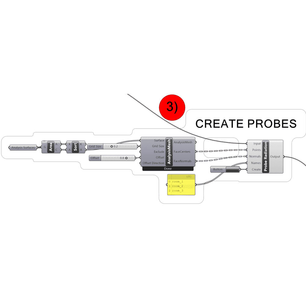
The Probe Radiation component takes its Input from the Solution component. The Points and Normals should be a Tree/List of points and vectors, where we want to get the daylight results. On Compute we call them the Probe Points.

We can generate the probe points with the AnalysisMesh component. We give the component a list of Surfaces, a Grid Size and an Offset height. The component then generates a mesh, a list of points for each face center of the mesh, and a list of normals associated with those points.

In this case we have 3 rooms, and we want to be able to distinguish those rooms from each other. That is why we give a list of surfaces to in the Surface input. That way the points and normals are separated into different branches. On Compute we call each branch a Probe Set. We can also give our probe sets names, by providing a list of names to the Names input in the Probe Radiation component.

Just as with the surfaces, it is important to check that your normals of the analysis mesh points in the right direction. The normals should point upwards.

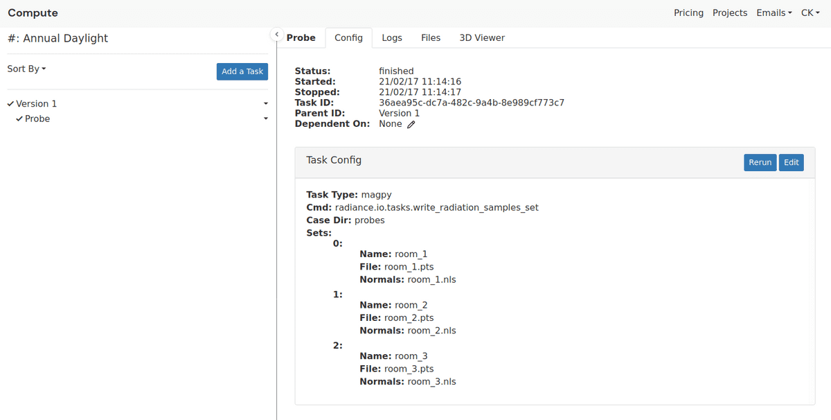
To create the Probe task we click the Create button. You can the go to the browser and see that a Probe task is created in your project as a child of the Version 1 task. The Probe task ussually run really fast, as it just turns the points and normals we created into a format that Radiance can understand.

Create Simulation Task

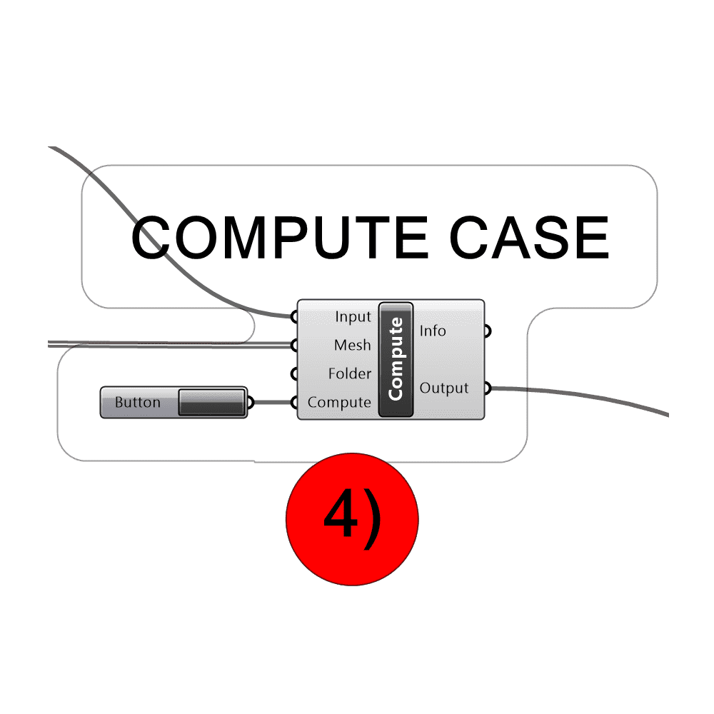
After the probes have been created it is time to click the Compute button! The Compute component takes the input from the Radiation Probe component and the meshes we defined in the beginning.

After clicking Compute two new tasks will appear in the project on Compute: Actions and Three Phase. The Actions takes the Rhino geometry, the names we gave the geometry and the material assignments, and turn them into Radiance scene files (.rad)

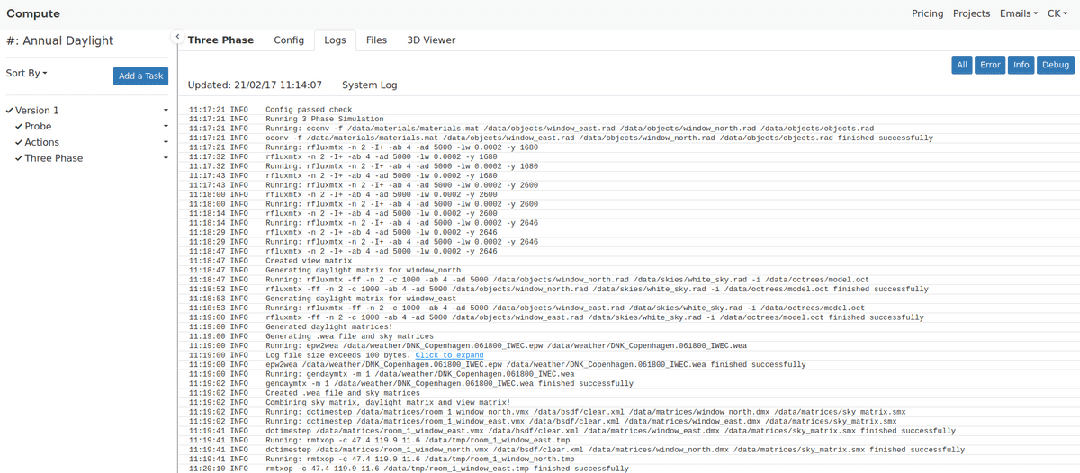
The Three Phase task is the actual simulation task. You can click on Logs to see the progress of the simulation. We stream all the logs back to you, so you can see what is happening.

You can also ready more about the Logs pane here

With 2 CPUs this demo case takes about 10min to simulate.

Create Daylight Metric Task

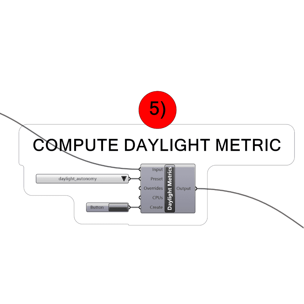
While the simulation is running we can create the Daylight Metric task. We do that with the Daylight Metrics component. It takes the output from the Compute component as its input, a preset of which metric we want to calculate. You can also change the number of CPUs to use (default is 1 CPU) and apply some overrides to the metric.

In this tutorial we are just going to pick the daylight_autonomy preset, but you can pick between:

• Daylight Autonomy
• Continuous Daylight Autonomy
• Spatial Daylight Autonomy
• Useful Daylight Illuminances
• Statistics

If you are interested you can read more about each Daylight Metric here and what overrides can be applied.

Download Results

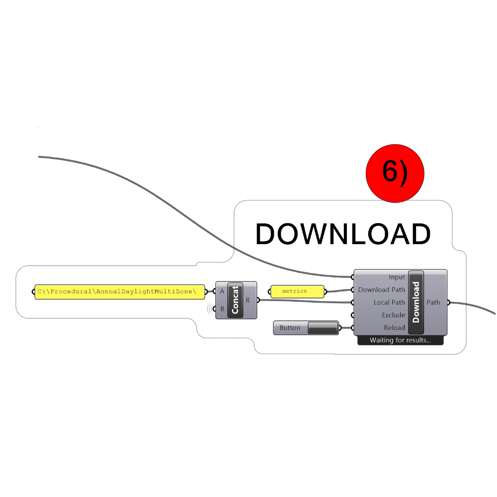
When both the Three Phase and Daylight Autonomy task is done we can download them, so they can be visualized in Grasshopper. We provide the download component with the output from the Daylight Metric task, the folder on Compute that we want to download and a Local Path that we want to download the results to. The component will itself start downloading the files as soon as they become available on the server.

The Download Path is the path on the server you want to download. The daylight metric results are saved at metrics. In case you want to download something else, you can takes a look at the Files tab to see which files are available.

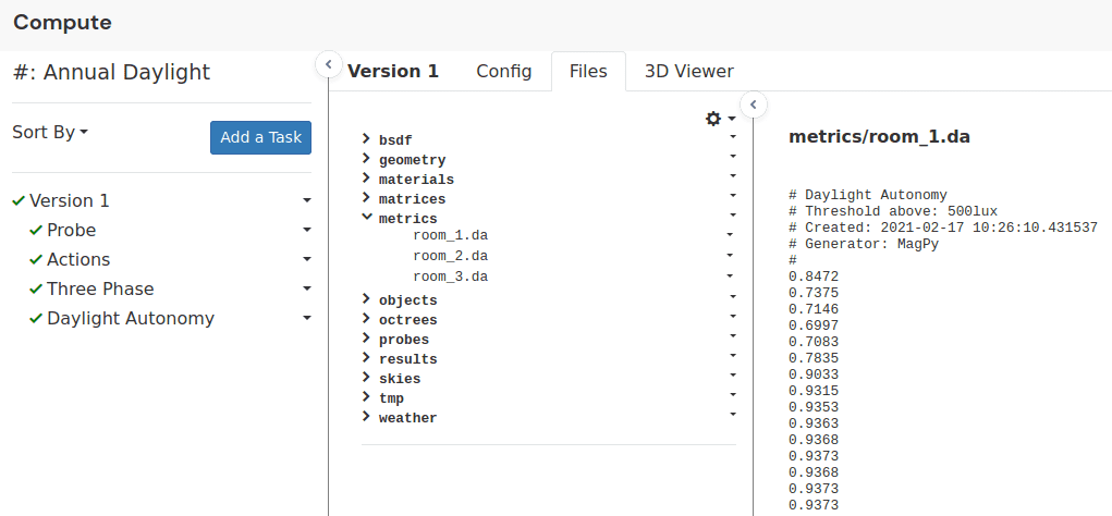
We can then feed the path we download the files to into the Radiation Results component, which will load them, and we can then visualize.

Final Results

The final results looks something like this